Algorithms

What is an algorithm?

An algorithm is a finite set of instructions that, if followed, accomplishes a particular task. In addition, all algorithms must satisfy the following criteria:

1. Input. Zero or more quantities are externally supplied.
2. Output. At least one quantity or result is produced.
3. Definiteness. Each instruction is clear and unambiguous.
4. Finiteness. If we trace out the instructions of an algorithm, then for all cases, the algorithm terminates after a finite number of steps. (Termination!)

We can also add “effectiveness”: every instruction must be basic enough and feasible. Ideally a person using only pencil and paper should be able to carry it out.

• Algorithms: always produce a correct result.
• Heuristics: may usually do a good job, but without providing any guarantee.

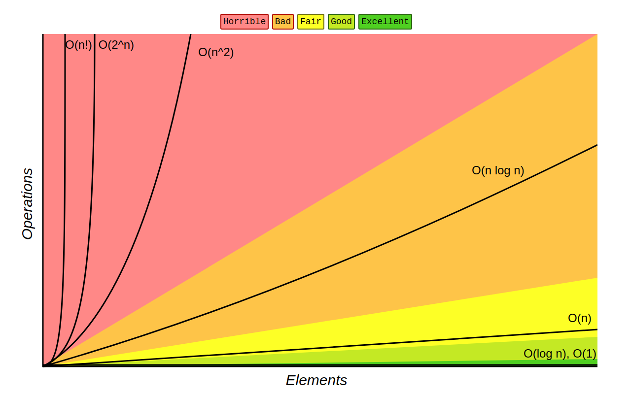
Function growth

$n! \gg 3^n \gg 2^n \gg n^3 \gg n^2 \gg n\log{n} \gg n \gg \log{n} \gg 1$

Space complexity

The space complexity of an algorithm is the amount of memory it needs to run to completion. The space needed for the algorithms is seen to be the sum of the following components:

1. A fixed space part that does not depend on the characteristics of the algorithm inputs and outputs. This part includes instruction space (i.e. the space of the code, space for static variables and constants, etc.)
2. A variable space part consists of the size of the variables which depend on a particular problem instance being solved: the space needed by allocated and referenced variables, and the recursive stack space.

When analyzing the space complexity of an algorithm, we concentrate solely on estimating the variable part.

Any time memory is allocated dynamically, whether through manual allocation or by adding levels to the stack there is the possibility the space complexity of the algorithm will increase.

When given a choice between best or worst time complexity, usually the worst is more useful.

Time complexity

The time complexity of an algorithm is the amount of computer time it needs to run to completion. A program step is a meaningful segment of a program. Although simple operations like addition or multiplication can take different time on a particular machine, we consider such primitive operations as single steps $\rightarrow$ then we can count the number of program steps.

Example: return a+b+b*c+(a+b-c)/(a+b)+4.0; can be considered to take only 1 step.

An assignment statement (with no calls to other functions) takes 1 step. Simple control statements (like if, else, switch with no calls to other functions in the condition) take 1 step. More complex control statements (for, while, and repeat loops for example) we consider the step counts only for the control part of the statement.

In a for loop there are 2 considerations to make:

1. The cardinality of the set: $\text{last element index} - \text{first element index} + 1$
   • Example: $S= \{1, 2, \ldots, n\} \rightarrow \text{cardinal}(S) = n-1 +1=n$
2. The breaking condition of the for loop. This must be tested 1 extra time for the program to leave this code behind.

Example

Statement	Steps/execution (s/e)	Frequency	Total steps
1. Algorithm Sum(a, n)	$0$	$-$	$-$
2. s := 0	$1$	$1$	$1$
3. for i = 1 to n do	$1$	$n + 1$	$n + 1$
4.     s := s + a[i]	$1$	$n$	$n$
5. return s;	$1$	$1$	$1$

Total	Big-Oh
$2n + 3$	$\mathcal{O}(n)$

Sorting

Applications of sorting:

• Searching (for sorted data, searching takes just log n time)
• Closest pair: among n numbers, which pair have the smallest difference between them?
• Element uniqueness: Are there any duplicates in a given set?
• Frequency distribution: Given a set of n numbers, which element occurs the largest number of times?
• Selection: What is the kth largest number in an array?

Algorithm design tools

(Loop) invariant

In an iterative algorithm, a loop invariant is a property that is maintained throughout the computation. In recursive design it's just called an invariant. It is usually an easier or smaller instance of the final problem you are trying to solve which the algorithm expands at each iteration until you have solved the entire problem. This can also be used to prove the correctness of an algorithm.

Divide and conquer

Recursively breaks a problem into smaller subproblems, solves them independently, and combines their solutions to form the overall solution.

Tail recursion

Tail recursion can be used to remove multiple recursive calls in a recursive algorithm implementation, thereby significantly shrinking the tree size. See tail recursive fibonacci on the fibonacci page.

Recurrence relations

Recurrence relation solution	Algorithm	Big-Oh
$T(n) = T(n/2) + \mathcal{O}(1)$	Binary search	$\mathcal{O}(\log{n})$
$T(n) = T(n-1) + \mathcal{O}(1)$	Recursive sum	$\mathcal{O}(n)$
$T(n) = 2 T(n/2) + \mathcal{O}(1)$	Tree traversal	$\mathcal{O}(n)$
$T(n) = T(n-1) + \mathcal{O}(n)$	$n^2$ sorting algorithms	$\mathcal{O}(n^2)$
$T(n) = 2 T(n/2) + \mathcal{O}(n)$	Merge sort (& average case quicksort)	$\mathcal{O}(n\log{n})$
$T(n) = 2 T(n-1) + \mathcal{O}(1)$	Binary (search) tree construction	$\mathcal{O}(2^n)$